Generating a velocity profile for a mobile robot

This post is based on my M.Sc. thesis, the goal of which was redesigning the velocity profile generator of an autonomous mobile robot. The velocity profile can be used to plan and optimize a robot’s movement.

What is a velocity profile?

A velocity profile is a depiction of speed as a function of time or distance. A velocity profile for a known route can be created in advance if the restrictions of the route and the robot are known. An autonomous mobile robot can use a pre-made velocity profile as its speed setpoints and thus optimize its movement.

What is required for a velocity profile?

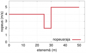
A velocity profile can be created based on a known route and other restrictions. A simple route consists of straight lines and turns. In general, the robot must move more slowly at turns than on a straight route, so that it does not, e.g., fall or slip sideways. Based on the shape of the route, or its geometry, a speed control function, i.e., a description of the maximum speed for each part of the route, can be created. In the figure below, the velocity limit is 4 m/s for the first 20 meters, then 2 m/s for 5 meters and finally 5 m/s for 20 meters.

Other restrictions include the properties of the robot, such as its center of gravity, engine power and tire properties. In addition to velocity limits, these restrictions have been simplified into maximum and minimum values of acceleration (the derivative of velocity, i.e., how quickly the speed is allowed to change) and jerk (the derivative of acceleration, i.e., how quickly the acceleration is allowed to change).

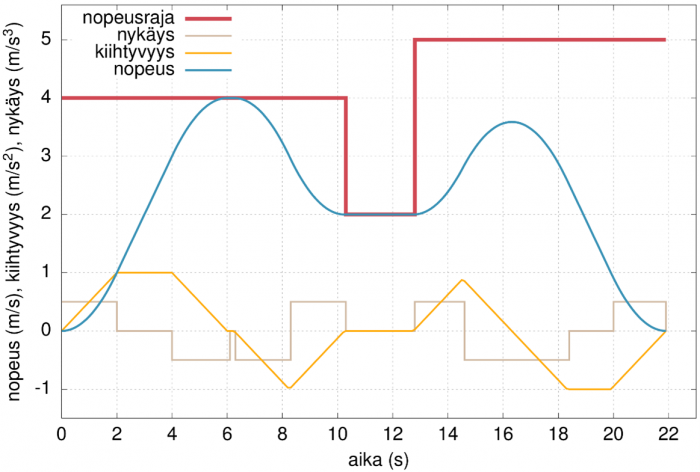
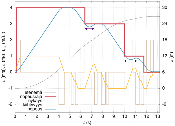
Once the speed control function, acceleration and jerk are known, a velocity profile can be created based on them. A velocity profile can be created and presented in several different ways. In the figure below, the velocity profile is shown as a function of time. The speed control function, acceleration and jerk are also plotted on the graph.

Why is the existing generator being replaced?

The velocity profile generator is intended to work as part of existing, more comprehensive robot automation software. The current velocity profile generator used in the software is written in C++, a general-purpose, statically typed programming language that supports object-oriented programming and dynamic memory management. The execution of the generator is complicated and prone to errors; memory management in particular requires caution to avoid serious errors.

The existing algorithm creates velocity profiles analytically, i.e., it creates different polynomials that form the velocity profile. For example, in the figure above, the velocity function is a second-degree polynomial in the time interval of 0–2 s, a first-degree polynomial in the time interval of 2–4 s and, again, a second-degree polynomial in the time interval of 4–6 s. After reaching the velocity limit, it is constant for a short time.

Since the execution of the generator is difficult to understand and the analytical method of generation and presentation is unnecessarily complex for the need, it was decided that a new generator be made instead. The language chosen for this purpose was Haskell, an (almost) purely functional, statically typed and lazily evaluated programming language.

Different ways of generating and presenting velocity profiles were studied for the new velocity profile generator. A velocity profile can be presented as a list of discrete points instead of a function; each point contains at least a velocity value and a value for time or progression. There were several options for the velocity profile generating algorithm, and we selected a “bungee rope algorithm” that works in a simple way: it increases the velocity of the profile points slightly over many iterations and tries to keep the profile within the limits provided.

What is the new velocity profile generator like?

During one iteration, the new algorithm goes through the points in the velocity profile and attempts to increase each point’s velocity once. When one point attempts to increase its velocity, it asks the previous two and next two points if they accept the increase in velocity. The other points can answer no, yes, or yes if the point being surveyed can also change its velocity. The survey can also go further in the profile. When one point eventually answers just yes or no, the other points will either make the changes in their speed or make no changes at all. The review will continue from the next point that has not changed its speed.

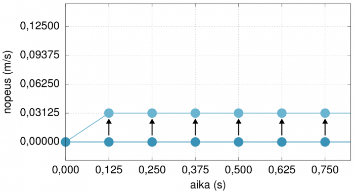
The figure below shows an example of the first points in the profile and the first iteration, where the (smallest) speed increase step is 0.03125 m/s and the time step is 0.125 s. No point objects to increasing the speed.

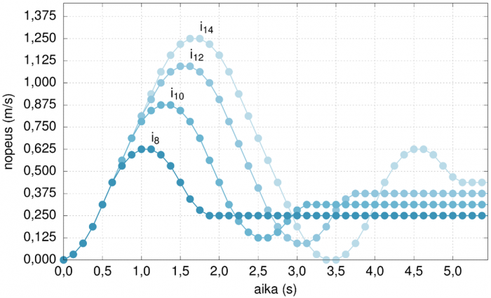
The new algorithm aims to increase the speed as much as possible as quickly as possible and to keep the speed as high as possible for as long as possible even if the speed of the next points in the profile needs to be reduced. This functionality results in rippling at the beginning of the iteration and “dips” in the final velocity profile.

The figure below shows a ripple forming during iterations 8, 10, 12, and 14.

In the figure below, the “dips” in the final profile are marked with purple arrows.

Summary

The new velocity profile generator produces relatively good velocity profiles, and the profiles comply with acceleration and jerk limits and almost all velocity limits. The algorithm does, however, require some further development.

---